Category: Computer Science

  • The beauty of dynamic programming

    I just discovered dynamic programming and damn, I’m blown away by the concept.  The other day, hile working through a homework assignment, I compared the run times between two python functions that I wrote, one function written recursively and the other written in a dynamic programming fashion.  Starting with the recursive solution, I arrived at the following:

    def fibonacci(n):
        if n == 0:
            return 0
        if n == 1:
            return 1
        return fibonacci(n-1) + fibonacci(n-2)
    

    That’s a fairly standard implementation of Fibonacci. There are two base cases; n=0; n=1.  So when n is either of these two numbers, the function simply returns 0 or 1, respectively.  But for any other number, the function recursively calls itself until reaching the aforementioned base cases.

    So far so good, right?  And for calculating small values of n, this implementation doesn’t really present a problem. But say we want to calculate fibonacci when n equals 40. How long does this take? Alarmingly, this computation hovers around 45 seconds:

    ./fibonacci.py 40
    fibonacci(40) = 102334155 took 45.22154 seconds
    

    Now, what if we run the same calculation. But this time, we run it using a dynamic programming technique? How much time does that shave off?

    ./fibonacci.py  --dynamic-programming 40
    fibonacci(40) = 102334155 took 0.00002 seconds
    

    What ?! From 45 seconds down to under a millisecond ?! How is that possible?

    def fibonacci_dynamic_programming(n):
        fibonacci = [0,1]
        for _ in range(0, n):
            fibonacci.append(fibonacci[-1] + fibonacci[-2])
        return fibonacci[n-1] + fibonacci[n-2]

    As you can see from the code above, instead of recurisvely calling fibonacci, we iteratively calculate all the values. In other words, this implementation runs linearly (i.e. direct proportion to n), unlike the first, recursive implementation, which runs exponentially.


  • Wrapping up discrete mathematics course

    Last Friday, I took the final exam for my (distant learning) discrete mathematics course and just now I had logged into the student portal (i.e. Blackboard), surprised to find that my exam had not only been graded but my final grade had been posted as well. I finished the course with an 88%, a B, a few points short of an A.  In the past, I would’ve incessantly beat myself up over not achieving the highest grade, denigrating myself with self destructive thoughts: if only I tried harder … if only I studied more … if only I was smarter …

     But not this time.

    This time, I’m inhibiting those thoughts. Instead, I’m celebrating. Celebrating that I’m fortunate enough to be able to take this mathematics course, a course where I learned about: writing proofs, solving Diophantine equations, applying set theory, counting with modular arithmetic, proving assertions with mathematic induction, converting recursive functions into closed form functions using characteristic equations method. Prior to the course, I was never exposed to those concepts.  Looking back, I only vaguely heard of those terms.  And who knows if I get to apply any of those concepts as I pursue a master’s – maybe a PhD, one day. Who knows if I’m lucky enough to apply that knowledge to my job as a software engineer.

    But who cares?  Because really, my goal was to stretch myself, learning more about my field and craft: computer science.

  • Graph theory and upcoming final exam

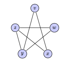
    I just scheduled my final exam for my discrete mathematics course, now that I submitted my homework for the final assignment covering graph theory. Throughout this assignment, I was introduced to a variety of concepts: Leonard Euler and his discovery of Euler paths and circuits, Hamiltonian paths and circuits, and a handful of graph related terminology (e.g. vertex, edges, degrees, bridge, cut-vertices, isomorphic graphs, trees, forests).

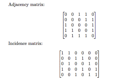
    In addition to the concepts above, I learned two different ways to represent graphs in (computer) memory. One approach is using adjacency matrix, a matrix whose columns and rows are represented by each vertex. The second way to represent a graph is by an incidence matrix; unlike an adjacency graph, an incidence matrix’s columns are vertices, the rows representing edges.

    Star like graph
    Star like graph
    Adjancey and Incidence matrix
    Two ways to represent the (above) graph

    Although the lesson only scratched the surface on graph theory, I reveled in the fact that many of the terms I learned were actually terms that I encountered at work, terms that I had no idea were rooted in mathematics.

    For example, the term forest (in graph theory) is defined as a collection of trees; I encountered this term while working as a system administrator, a time when I managed Active Directory (a centralized authentication system) and all the security rules and policies bound to a forest.

    In addition to the example above, I find comfort in the fact that some data structures (e.g. binary search tree) and algorithms (e.g. breadth first search) that I’ve studied in the past build on top of graph theory.

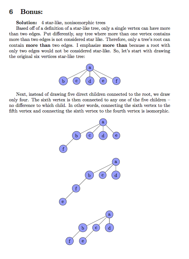
    Star-like graphs that are nonisomorphic
    Star-like graphs that are nonisomorphic

    In any case, I really enjoyed learning about graph theory, a lesson I’ll continue to build on top of as I pursue my life long study of mathematics and computer science.

  • Software and system ownership

    Although I sometimes find getting paged for operational issues enervating, I wouldn’t have it any other way.

    It’s well known that software engineers at Amazon (Web Services) own their systems, end to end. This means that we not only develop and maintain our software, but we operate the underlying system, complete ownership.

    From a software point of view, one can run into an infinite number of issues. Got a build error? Roll up them sleeves and start digging through the compilation errors.  You committed some code that broke the build? Fix or rollback the changes. You defined a dependency that’s deprecated? Update the dependency and ensure your unit and integration tests pass.

    Similarly, we maintain the underlying system. If we deploy our systems to a servers, physical or virtual (e.g. EC2), we must keep it alive, like a breathing entity. From checking disk performance, to checking heap allocation, we monitor our systems closely, configuring monitors to alarm us when any component misbehaves.

    In other words, there’s no divide between development and operations. There’s no separate team that handles operational issues, no DevOps. There’s no nonsense like writing our software and then chucking it over to another group to deploy it, a group that would otherwise find it annoying at best and frustrating at worst.  Because I’ve been in those positions, where I’m on the hook for deploying software that I cannot fix. Similarly, I’ve been in situations where the deployment fails and then I must ring in someone who’s more familiar with the code base.

    But now, I’m in a position where I’m responsible for the code I write.

    Why is this important?

    Although some would argue that software developers should stick to software development, and that there should be a clear separation of duty, I believe that owning a system end to end promotes operational excellence and a sense of ownership.


  • Where discrete mathematics meets an interview question

    Last week, I was sitting behind my desk at work, surfing hacker news and and at the top of the website floated an article by the co founder of “Daily Coding Program”, a small tech start up that e-mails daily newsletters with a programming question.  The article shared some of their insights over the past year and how they bootstrapped the company and eventually grew to $2,000 in monthly revenue.

    Although I was interested in reading the blog post, I ended skipping over most of it and navigated to their front page, where I scrolled up and down and read more about the company’s product.  When I reached the end of the front page, I was confronted with a sample interview question:

    There’s a staircase with N steps, and you can climb 1 or 2 steps at a time. Given N, write a function that returns the number of unique ways you can climb the staircase. The order of the steps matters.

    This question, I had initially thought, could be solved using some techniques that I recently learned from taking my discrete mathematics course. But to confirm whether or not I could apply permutations and combinations, I hollered at my colleague, repeating the question out loud and asking him how this problem could be solved. And as I started reading the question out loud, “There’s a staircase with N steps, and you can climb …” he interrupted me, finishing my sentence with, “1 or 2 steps at a time.”

    Apparently, while preparing for interviews with Google and Microsoft, he had stumbled across this same practice problem.

    So after letting him interrupt me, I asked him if this particular problem could be solved with permutations or combinations. In other words, do these two mathematical concepts apply to the problem. He confidently answered, “No — dynamic programming.” He then proceeded to step me through his solution, scribbling down his work on a white piece of 8.5 x 11 that sat on my desk.

    Fast forward to now.

    I’m at home, starting the next lesson for my discrete mathematics course, the lesson title: “Counting using Recurrence Relations” and “Solutions to Recurrence Relations.” I’m skimming the chapter, building a mental model of what the entire chapters entail, an overview.  And when I reached the end of the first chapter, where exercise problems live, I couldn’t help but form a little grin.

    To my surprise, the following chapters cover topics relating to the interview question that I had just read. In fact, the exercise in the chapter is phrased almost identically:

    Sal climbs stairs by taking either one, two, or three steps at a time. Determine a recursive formula for the number of different ways Sal can climb a flight of n steps.

    So, I find it always nice and serendipitous when what you are learning, either in school or on your own, can be applied to real life examples. Albeit, this application was only for an interview question.

    But I’ll still consider that as a victory.


  • Lessons learned coding the quicksort algorithm in assembly (i.e. MIPS)

    About six months ago, I enrolled myself in a computer organization (i.e. CS1410) course offered by University of Northern Iowa and I’m taking it remotely from Seattle, where I work full time as software engineer at Amazon (Web Services).

    I’ve completed about two thirds of the course, which consists of sixteen homework assignments and three proctored exams, my most recent homework assignment requiring me to code in MIPS, a low level programming language known as assembly. More specifically, I’m tasked with implementing the quicksort, a recursive algorithm, to sort a sequence of integers.  This homework assignment targets teaching two important computer science concepts: the run-time stack and calling conventions.

    Normally, I complete one homework assignment per week. However, this homework assignment was extremely challenging, taking roughly two and a half weeks to complete. The first couple days I dedicated to drilling the quicksort algorithm into my head, ensuring that I could visualize how the program actually sorts elements in the sequence, reading article after article (and sections from the books that have been collecting dust on my bookshelf); the remainder of the time I spent deep diving into writing the assembly code, typing code and executing in a MIPS simulator.  I cannot explain the number of times I grew frustrated, banging my head into the keyboard, because of program crashing.  At one point, I was stuck — for three days straight. None of my troubleshooting skills pinpointed me to the root cause.  After three days of staring at the code, I finally discovered the problem: I was corrupting the run-time stack.  After modifying one single line, updating the instruction to subtract 24 instead of adding 24 to the stack pointer (i.e. $sp register), the quicksort program ran flawlessly.

    All in all, I found the homework assignment as challenging but rewarding.


  • A brief introduction to cache organization

    As a software programmer, I always had a vague understanding of how an operating system fetches data from memory.  At an abstract level, I understood that a processor requests data from the memory controller, sending a message (with the memory address encoded) across the bus.

    But I learned recently that in addition to the system’s physical memory—the same memory I used to squeeze into the motherboard when installing RAM—there are multiple hardware caches, completely abstracted from the programmer.

    These caches sit between the processor and main memory, called: L1 cache and L2 cache and L3 cache.  Each cache differs: in cost, in size, and in distance from the CPU. The lower the digit, the higher cost, the smaller in size, and the closer it sits to CPU.  For example, if we compare L1 and L2 cache, L1 costs more, holds less data, and sits closer to the processor.

    When the processor wants to retrieve data from memory, it sends a request first lands in L1 cache’s world.  If L1 has that memory page cached, it immediately sends that data back to the processor, preventing the request from unnecessarily flowing towards the memory controller.  This pattern of checking local cache and forwarding requests repeats until the request eventually reaches the memory controller, where data is actually stored.

    The further we allow the CPU’s request to travel down the bus, we penalize the CPU, forcing it to wait, like a car at a stop sign, for longer cycles. For example, the CPU waits 4 cycles for L1 cache, 12 cycles for L2, 36 cycles for L3, and—wait for it—62 cycles when accessing main memory.  Therefore, we strive to design systems that cache as much data as possible and as close to the CPU, increasing overall system performance.

    We break down a cache into the following components:

    • Blocks
    • Lines
    • Sets
    • Tag
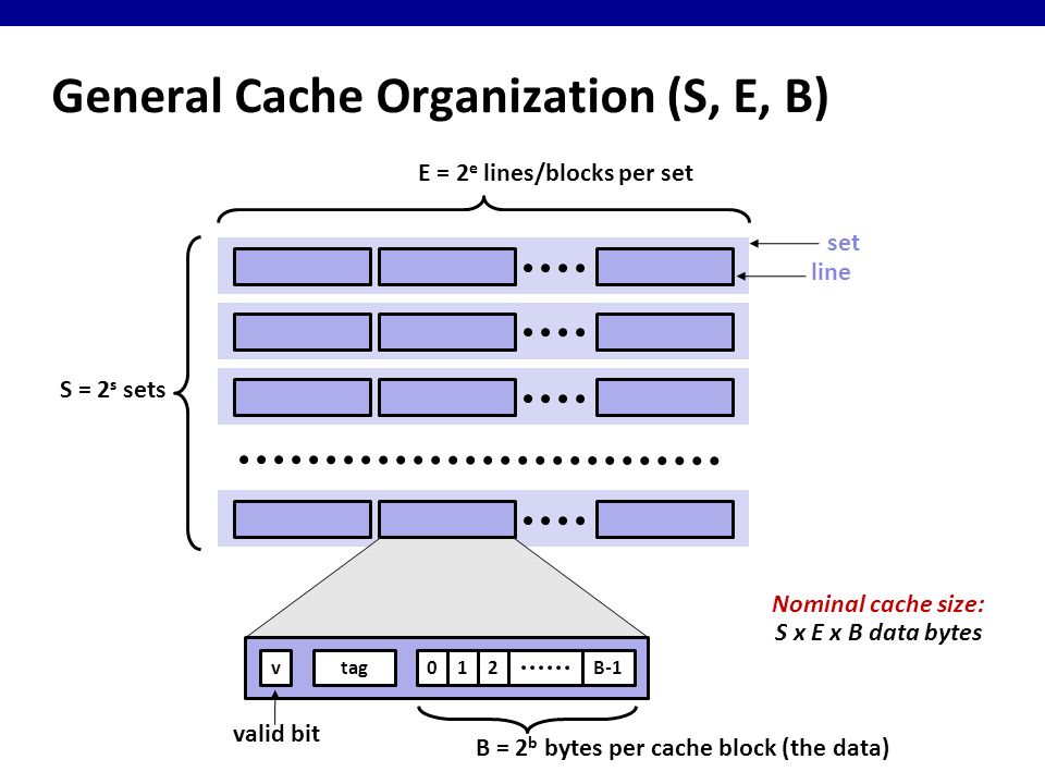
    sets, lines, blocks
    Cache organized into sets, lines, and blocks

    As you can see from the image above, we organize our cache sets (S), lines (L), and blocks (B).  One block of data represents 8 bits (1 byte) and every block of data is represented by a physical memory address. For example, the memory address 0x0000 may store 010101010 and 0x0001 may store 01110111 another.  We group these blocks together into a line, which store sequential blocks.  A line may store two or four or eight or sixteen bytes—it all depends on how we design the system.  Finally, each line belongs to a set, a bucket that stores one or more lines.  Like the number of bytes a line stores, a set can store one or two or three or forty—again, it all depends on our design.

    Together, the total number of sets, number of lines, and number of bytes determine the cache’s size, calculated with the following formula: cache size = S x E x B.

    In the next post, I’ll cover how a cache processes a memory address, determining whether it retrieves memory from cache or forwards the request to the next cache (or memory controller).

  • Defusing a Binary Bomb (phase 1)

    http://blog.itsmemattchung.com/2017/02/28/csapp-defusing-the-bomb-phase-1/

    I password protected the original post (email me for the password if you are interested in reading it).  When I posted the original link on reddit/r/compsci, multiple commenters suggested that I delete the article to avoid students from cheating (which was not my intention).  I then sent an e-mail to the professors (at CMU) and they kindly replied, asking me to remove the post:

    Matt,

    Thanks so much for your kind words. It’s great to hear that the book is helpful to you. While every student gets a slightly different bomb, the solution strategies for each phase are very similar. So it would be good if you could remove those posts.
    Thanks!
    Dave
  • Protected: Defusing a Binary Bomb (phase 1)

    This content is password protected. To view it please enter your password below:

  • How does the modulus operator work?

    As a programmer, I’ve written a line or two of code that includes the modulus operator (i.e. “return x % 2“).  But, never have I paused to think: “How does the underlying system carry out this operation?” In this post, I limit “underneath the hood” to the lowest level (human readable) programming language: assembly.

    So, I’ll take a program (written in C language) and dump it into assembly instructions. Then, I’ll explain each instruction in detail.

    My background in assembly programming

    Up until a few weeks ago, I had never studied assembly—I did flip threw a page or two of an assembly book, when a colleague mentioned, about five years ago, that his uncle programmed in assembly—and I certainly underestimated the role that assembly plays in my career.

    Sure—the days of writing pure assembly language evaporated decades ago, but the treasure lies in understanding how programs, written in higher level languages (e.g “C, Perl, PHP, Python”), ultimately boil down to assembly instructions.

    Modulus program

    So, I contrived a trivial modulus program written in C—let’s dissect it:

    // modulus.c
    
    int modulus(int x, int y){
        return x % y;
    }

    Converting C code into assembly

    Before a program can be executed by an operating system, we must first convert the program into machine code—we call this compiling.  Before we run our program (modulus.c) through the compiler, we need to discuss two arguments that we’ll pass to the compiler, in order to alter the default behavior.  The first argument, -0g, disables the compiler from optimizing the assembly instructions.  By default, the compiler (we’re using gcc) intelligently optimizes code—one way is by reducing the number of instructions.  The second argument, -S, instructs the compiler to stop at  just before it creates the machine code (unreadable by humans), and, instead, directs the compiler to create a file (modulus.s) containing the assembly instructions.

    # gcc -Og -S modulus.c
    

    The command above outputs a file, modulus.s, with the contents (unrelated lines removed):

    modulus:
    movl	%edi, %eax
    cltd
    idivl	%esi
    movl	%edx, %eax
    ret

    Let’s step through and explain each of the assembly instructions, one-by-one.

    mov

    When we want our CPU to perform any action, such as adding, substracting, multiplying, or dividing numbers, we need to first move bytes of data (an intermediate value, or from memory) to a register.  We move data to registers with the mov command, which is capable of moving data from:

    • register to memory
    • memory to register
    • register to register
    • immediate value to memory
    • immediate value to register

    The assembly above first moves data from one register (%edi) to another register (%eax).  This is necessary since subsequent instructions, such as cltd, rely on data being present in the %eax register.

    cltd

    cltd stands for “convert long to double long.”  But before we dig into why we need this instruction, we must detour and briefly explain the next instruction in line, idivl.

    When we send an idivl (divide long) instruction, the processor calcutes the numbers and store the quotient in one register, and stores the remainder in another.  These two values stored in the register are half the size; if the dividend is 32 bits, the cpu stores (1) 16-bit value in one register, and the other 16-bit value in another.

    Therefore, if we expect a 32-bit quotient and 32-bit remainder, then the dividend (which is, presumably, 32-bits) must be doubled—to 64-bits.  In our modulus program, we set a return value of type int.

    idivl

    idivil divides the numerator (stored in %eax) by the argument (or denominator) — the argument that we passed to the instruction.  In our assembly example above, idivl divides the value stored in %rax, by the value in %esi—x and y, respectively.

    movl

    At the end of a sequence, assembly (by default) returns whatever value is stored in the register %rax.  Therefore, the final instruction moves the remainder, not the quotient, from %edx to %rax.

    Wrapping up

    I hope I was able to share a thing or two on how a higher level program ultimately breaks down into simple assembly instructions.

    [1] I was banging my head against the wall until I found a easy to understand reason why we must convert long to double long: http://www.programmingforums.org/post12771.html