Category: Computer Science

  • Calculating page table entry size

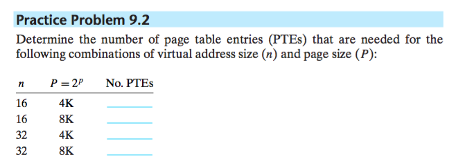
    How many page table entries are required given a virtual address size and page size?

    I was confronted with this question when reading Computer Systems from a programmer’s perspective on virtual memory management (VMM) which forced me to reread the chapter, over and over. It wasn’t until I forced myself to close the book, step away from the problem for a day, was I able to fully grasp what was being asked:

    Page table entries problem
    Page table entries problem

    Let’s narrow the scope and focus on a single instance, where n is 16 and P is 4K;  the question can be easily rephrased into something that makes more sense (to me): “How many 4k pages can fit into 16 bit memory address”?

    First, how any bits are required, for a 4K block size, to represent a single page? Well, 212 is 4096 so … that’s sufficient. Therefore, we can rephrase the abstract question that we can solve mathematically: “How many 12 bit pages can fit into a 16 bit virtual address size?”

    So, the problem now boils down simple division— 216 / 212,which can be expressed as 216-12: 24, which is sixteen (16). That’s 16 page table entries that required for a virtual address of size of 16 combined with a page size of 4k.

    The same approach can be taken for all the remaining practice problems. Convert the page (e.g. 4k, 8k) size into bits and divide that into the virtual address size (e.g. 16, 32)

  • A simple C problem

    I’m slowly working through “Computer Systems from a programmer’s perspective” [1] , struggling every bit of the way. I stopped beating myself up about it, though.

    The code snippets below are in C. The first function, inplace_swap, swaps two integers. The code itself looks lacks intent but I promise you, it swaps two integers.

    The second function, reverses an array. Coming from the Python world, I wondered why in the world we need to pass incount as an additional argument. I discovered the additional argument is absolutely necessary. C functions will always collapse array arguments into a pointer. The length of pointer, which is nothing more than a memory address, cannot be calculated [2].

    #include <stdio.h>
    
    void inplace_swap(int *x, int *y){
        *y = *x ^ *y;
        *x = *x ^ *y;
        *y = *x ^ *y;
    }
    
    void reverse_array(int a[], int cnt){
        int first, last;
        for (first = 0, last = cnt - 1; first <= last; first++, last--){
            inplace_swap(&a[first], &a[last]);
        }
    
    }
    

    This function appears to work just fine, at first. It reverses even numbered array flawlessly, however, fails to reverse an odd numbered array.

    void print_array(int a[], int cnt){
        int i;
        for (i=0; i < cnt; i++){
            printf(" %d", a[i]);
        }
        printf("\n");
    }
    
    int main(){
        int a[] = {1,2,3,4};
        int a_length = sizeof(a)/sizeof(int);
        printf ("Reversing 1 2 3 4 : ");
        reverse_array(a, a_length);
        print_array(a, a_length);
    }
    
    $ ./reverse_array
    Reversing 1 2 3 4 :  4 3 2 1
    
    int b[] = {1,2,3,4,5};
    int b_length = sizeof(b)/sizeof(int);
    printf ("Reversing 1 2 3 4 5:");
    reverse_array(b, b_length);
    print_array(b, b_length);
    
    $ ./reverse_array
    Reversing 1 2 3 4 5: 5 4 0 2 1
    

    3 practice problems

    The author reveals there is a bug and poses 3 questions:

    1. For an array of odd length cnt = 2k + 1, what are the values of variables first and last in the final iteration of function reverse_array?
    2. Why does this call to function xor_swap set the array element to 0?
    3. What simple modification to the code for reverse_array would eliminate this problem?

    In an odd length array, the variables first and last values are the same. This explains why the middle array element is set to 0. Any number XOR’d with itself will always produce 0. Here are a few examples of XOR’ing two binary values of the same value:

    0001 ^ 0001 = 0000
    0111 ^ 0111 = 0000
    

    I grew frustrated with the last question. For ten minutes, I held back my impulse to flip to the back of the book and reveal the solution. Instead, I slapped a piece of a piece of paper and a pen onto my desk, and stepped through the each iteration. There’s something about putting the pen to paper, that activates a different part of the brain.

    1 2 3 4 5
    5 2 3 4 1
    5 4 3 2 1
    
    1 2 3 4 5 6 7
    7 2 3 4 5 6 1
    7 6 3 4 5 2 1
    7 6 5 4 3 2 1
    

    The little fix

    In an array with odd number of elements, the middle item is always in its final position. We should never call inplace_swapfor the middle item. Instead, we change the condition in the for loop from first <= last to first < last.
    Footnotes

    [1] My colleague Richard – who graduated from Carnegie Mellon – recommended this book. Its the only book he read from to back, twice.
    [2] http://stackoverflow.com/questions/492384/how-to-find-the-sizeofa-pointer-pointing-to-an-array
  • Teaching as a form of learning: Binary Search Trees (BST)

    Last week, an e-mail was sent out to an internal mailing list [1], looking for volunteers to lecture on data structures & algorithms topics, but nobody replied. I jumped at the opportunity. I volunteered to lecture on binary search trees, without any previous knowledge on the topic. Why in the world would I volunteer to teach something that I know nothing about ? Well, one of the best ways to learn something is attempt to teach it. I love teaching as much as I love learning; teaching forces you to deeply understand the subject, internalize the material, and requires distilling the concepts into digestible bits and pieces. Here’s Ken Thompson’s advice [2].

    But I love teaching: the hard work of the first class, the fun of the second class. Then the misery of the third.

    —Ken Thompson

    In the post, I’m covering what a binary search tree is, its structure, and the basic operations: find, insert, and delete. We also cover the three methods for traversing the tree. At the end of this post are practice problems to help drive the concepts home.

    Next is an example problem that glues the concepts together.

    Example: Badging in & out of the office

    Picture an office requiring employees to badge in and out as they enter and exit the premise. We want to keep track of the employees in the building. We also want to be check if a specific employee is currently in the building. Let’s implement a binary search tree to maintain this dataset.

    As employees badge in, we insert the Employee object (using the employee ID as the key) into the three. When employees badge out, we remove them from the tree. Occassionally, we search the database asking “Is Employee X currently in this building?”

    Tree structure and performance

    What do binary search trees offer over other data structures [3] ?

    The binary tree data structure elegantly combines the flexibility and benefits of two existing data structures: linked lists and arrays. Linked lists efficiently add and delete nodes, by updating pointers, but inefficiently search. Linked lists require iterating over every node (i.e “from the head of the list”) until the desired node is found. Arrays, on the other hand, are perfect for searching – when taking advantage of the index – but are unsuitable for insertions/deletions. When inserting at a[i], all indexes greater than i must be shifted up; when an item is deleted at a[i], all indexes greater than i must be shifted down.

    This table compares the average runtime complexity of the three data structures.

    Data Structure Search Insert Delete
    Arrays O(1) O(N) O(N)
    Linked Lists O(N) O(1) O(1)
    BSTs O(logn) O(logn) O(logn)

    Binary search trees are suitable for specific problems. Binary search trees can be used to solve problems such as runway reservations [3]. Before we dive into the structure and implement the methods, let’s cover some terminology.

    Tree Terminology

    Here’s a visual representation of a binary search tree.

        15
       /  \
      7    21
     / \
    5  10
    

    A tree consists of nodes that are connected by edges. Those lines above represent the edges.

    • Path – Walking node to node, along the edges, creates a sequence known as the path.
    • Root – The node at the very top of the tree. There is only one root in the tree.
    • Parent – Every node, except for the root, has an edge connecting to the node above it.
    • Traversechecking or performing an operation on the node
    • Leaf – a node that contains no children
    • Level – The number of generations from the root node (level 0). For example, the root’s childrens are at level 1.

    Structure & Operations

    The structure of a tree is straight forward. It contains a reference to its root node, which is an instance of the Node class. TheNode class contains two references: leftChild, rightChild. The leftChild references a node whos key (i.e “used for comparing”) is less than the current node’s key, and rightChild references a node with a key greater than the current node’s key. This ordering restriction is a property of BSTs, but not all trees.

    Here’s some sample code of the data structure:

     public class BinaryTree<E> {
         Node root;
    
         private class Node<E> {
             int key;
             E data;
             private Node leftChild;
             private Node rightChild;
    
             @Override
             public String toString(){
                 String myString = "<Node [" + this.key + "]>";
                 return myString;
             }
         }
    }
    

    Searching

    Searching for the node is quite easy. Our method, find, accepts a key parameter. We start at the root. If the key we are searcing for is less than the node’s key, continue walking along the edge connecting to the leftChild. If the key is greater than the node’s key, continue walking along the edge connecting to the rightChild. When the key we are searching for is equal to that of the node, return the node.

    public Node<E> find(int key){
        Node<E> currentNode = this.root;
        while(currentNode !=null){
            if (currentNode.key == key){
                return currentNode;
            }
    
            if (key < currentNode.key){
                currentNode = currentNode.leftChild;
            } else {
                currentNode = currentNode.rightChild;
            }
        }
    
        return currentNode;
    }
    

    Inserting

    Inserting a node is a little more involved, but not by much. We apply an algorithm similar to find but we check our base condition is when the leftChild or rightChild is null.

    public void insert(int key, E data){
        Node<E> newNode = new Node<E>();
        newNode.key = key;
        newNode.data = data;
        if(root == null){
            root = newNode;
            return;
        }else{
            Node<E> currentNode = root;
            Node<E> parent;
            while(true){
                parent = currentNode;
                if(key < currentNode.key){
                    currentNode = currentNode.leftChild;
                    if (currentNode == null){
                        parent.leftChild = newNode;
                        return;
                    }
                }else{
                    currentNode = currentNode.rightChild;
                    if (currentNode == null){
                        parent.rightChild = newNode;
                        return;
                    }
                }
    
            }
        }
    }
    

    Traversing

    There are three ways to traverse a binary tree:
    • Pre Order
    • In Order
    • Post Order

    The most common of the three is in order. In our example code, we only print the currentNode.

    public void inorder(Node<E> localRoot){
    
        if(localRoot !=null){
            Node<E> currentNode = localRoot;
            inorder(currentNode.leftChild);
            System.out.println(currentNode);
            inorder(currentNode.rightChild);
        }
    
    
    }
    
    public void preorder(Node<E> localRoot){
        if (localRoot != null){
            Node<E> currentNode = localRoot;
            System.out.println(currentNode);
            preorder(currentNode.leftChild);
            preorder(currentNode.rigthChild);
        }
    }
    
    public void postOrder(Node<E> localRoot){
        if (localRoot != null){
            Node<E> currentNode = localRoot;
            postOrder(currentNode.leftChild);
            postOrder(currentNode.rightChild);
            System.out.println(currentNode);
        }
    }
    

    Deleting

    There are three cases we must consider when deleting a node:
    • node with zero children
    • node with single child
    • node with two children

    Let’s consider the first case whend deleting a node with zero children.

     Before               After
    
        15                  15
       /  \                /  \
      7    21             7    21
     / \                   \
    5  10                   10
    

    Delete with zero children

    We maintain a reference to the deleted node’s parent. We “delete” the node by updating the parent’s pointer (leftChild or rightChild) to null. The only edge case we consider is if the deleted node is the root. In thtat case, we just update root to null.

    public boolean delete(int key){
        Node<E> currentNode = root;
        Node<E> parent = currentNode;
        boolean isLeftChild = false;
    
        while (currentNode.key != key){
            parent = currentNode;
            if (key < currentNode.key){
                isLeftChild = true;
                currentNode = currentNode.leftChild;
            } else {
                currentNode = currentNode.rightChild;
            }
            // node not found
            if (currentNode == null){
                return false;
            }
        }
        // Case 1: No children
        if (currentNode.leftChild == null && currentNode.rightChild == null){
            if (currentNode == root){
                root = null;
                return true;
            }
            else if (isLeftChild){
                parent.leftChild = null;
                return true;
            } else {
                parent.rightChild = null;
                return true;
            }
        }
        return false;
    }
    

    Delete node with single child

    We just covered how to update the tree when a node has no children. Deleting a node, with a single child, is more involved, but just a little more. There’s four cases for the deleted node:

    • it’s the leftChild of its parent and has a leftChild
    • it’s the leftChild of its parent and has a rightChild
    • it’s the rightChild of its parent and has a leftChild
    • it’s the rightChild of its parent and has a rightChild

    In the first two diagrams, we are deleting node 7. In the last two, we are deleting node 21.

         Left child with single left child
    
        15                15
       /  \              /  \
      7   21            5   21
     /
    5
    
         Left Child with a single right child
    
        15                15
       /  \              /  \
      7   21            9   21
       \
        9
    
         Right child with single left child
    
        15                15
       /  \              /  \
      7    21           7    18
          /
         18
    
         Right child with single right child
    
        15                15
       /  \              /  \
      7    21           7    25
             \
              25
    
    if (currentNode.leftChild != null && currentNode.rightChild == null){
        if(currentNode == root){
            root = currentNode.leftChild;
        }
        else if(isLeftChild){
            parent.leftChild = currentNode.leftChild;
        } else {
            parent.rightChild = currentNode.leftChild;
        }
    }
    else if(currentNode.rightChild != null && currentNode.leftChild == null){
        if (currentNode == root){
            root = currentNode.rightChild;
        }
        else if(isLeftChild){
            parent.leftChild = currentNode.rightChild;
        }
        else {
            parent.rightChild = currentNode.rightChild;
        }
    }
    
        15                15
       /  \              /  \
      7   21            8   21
     / \               / \
    5   9             5   9
       /
      8
    
        15
       /  \
      7   21
     / \
    5   9
         \
         12
        /  \
       10   14
    

    When deleting a node, we replace the node with its inorder successor. The successor is the minimum node, within the deleted node’s right child subtree. Take a moment and think about that. Why the right subtree, and not the left?

    Would the next largest number ever be to the left of the current node? No. By definition, all nodes to the left are less thanand all node to the right are greater than. Therefore, the smallest number (greater than the current node’s key) will be the minimum node, to the right.

    Once we identify the successor, we update the successor’s parent leftChild pointer with the successor’s rightChild pointer (this may be null). We finalize the connections by updating the successor’s rightChild pointer to the delete node’s rightChild.

    public Node<E> getSuccesor(Node<E> toBeDeleted){
    Node<E> parentSuccessor = toBeDeleted;
    Node<E> successor = toBeDeleted;
    Node<E> currentNode = toBeDeleted.rightChild;
    while(currentNode.leftChild != null){
        parentSuccessor = successor;
        successor = currentNode;
        currentNode = currentNode.leftChild;
    }
    if(toBeDeleted.rightChild != successor){
        parentSuccessor.leftChild = successor.rightChild;
        successor.rightChild = toBeDeleted.rightChild;
    }
    return successor;
    

    Drawbacks

    The binary search tree sounds like the dream, so why use an alternative data structure?

    My manager shared a story of an interview candidate who inserted a sequence of sorted items into a binary search tree. Pause for a moment and visualize the data structure. What do you get?

    A linked list!

    This increases the height of the tree and we lose advantage of the O(logn) performance. Binary Search tree is suited best forrandomized keys, not sorted.

    Example

    public class Employee {
        private int id;
        private String firstname;
        private String lastname;
    
        public Employee (int employeeid, String firstname, String lastname){
            this.id = employeeid;
            this.firstname = firstname;
            this.lastname = lastname;
        }
    
        @Override
        public String toString(){
            // < 05: Joe Schmoe >
            String myString = "< " + this.id + " " + this.firstname + " >";
            return myString;
        }
    
        public static void main(String[] args){
            Employee jboyd = new Employee(15, "jess", "boyd");
            Employee mstreiter = new Employee(7, "myles", "streiter");
            Employee mdavis = new Employee(21, "matt", "davis");
            Employee mmadsen= new Employee(5, "martin", "madsen");
            Employee mchung = new Employee(19, "matt", "chung");
    
            BinaryTree<Employee> employees = new BinaryTree<Employee>();
            employees.insert(jboyd.id, jboyd);
            employees.insert(mstreiter.id, mstreiter);
            employees.insert(mdavis.id, mdavis);
            employees.insert(mmadsen.id, mmadsen);
    
            // Is myles in the building?
            // returns true
            System.out.println(employees.find(mstreiter.id));
    
            // Jess clocks out
            employes.delete(jboyd.id);
    
            // Is Matt in the building?
            // returns false
            System.out.println(employees.find(mchung.id));
    
        }
    }
    

    Exercises

    1. Write a function that verifies that a binary search tree is valid.
        15
       /  \
      7   21
     / \
    5   17
    

    Acknowledgements

    Thanks to Jess Boyd for correcting my initial draft, Matt Davis for pointing out the drawbacks of BSTs, and Martin Madsen for techniques to make the post more comprehensible.

    Footnotes

    [1] In a previous post, I shared how I am teaching myself data structures and algorithms. In the breakroom work, a colleague overheard a group forming to study together – the weekend bravehearts. I was lucky enough to catch the group at the head end. We meet Friday after work, and Saturday mornings. If you live in the greater Seattle area and wanted to join, e-mail me and I’ll bring you along.
    [2] This is a quote pulled from interview, from the book “Coders at work”, with Ken Thompson
    [3] (1, 2) MIT’s lecturer presents a scheduling problem and compare the advantages and disadvatages of previously discussed datastructures (e.g “linked lists”, “arrays”, “heaps”). I recommend watching it:https://www.youtube.com/watch?v=9Jry5-82I68
  • Python progression path – quiz

    Python progression path – From apprentice to guru is a popular StackOverflow post. To categorize whether a person should take his beginner/intermediate course, one of the commentors posted this question:

    python progression quick

    I can better answer this question after reading Fluent Python. Example 1 and Example 2 deal with immutable and mutable data types – respectively. Let’s address each example individually.

    Example 1

    The id built in method returns the object’s memory address. We’ll use this to inspect the memory address for x and ythroughout the examples.

    x and y point to the same memory address when they are first assigned.

    >>> x = 42
    >>> y = x
    >>> id(x)
    4298172632
    >>> id(y)
    4298172632
    

    Because the value of x is immutable (e.g INT) and cannot be modified, by definition, a new memory address is allocated when x is modified. But, y‘s memory remains unmodified:

    >>> x = x + 1
    >>> id(x)
    4298172608
    >>> id(y)
    4298172632
    >>>
    

    Example 2

    Like Example 1, the memory address starts off the same:

    >>> x = [1,2,3]
    >>> y = x
    >>> id(x)
    4299948256
    >>> id(y)
    4299948256
    

    Now that we are dealing with mutable data types, x can be modified in place and the memory address does not change:

    >>> id(x)
    4299948256
    >>> id(y)
    4299948256
    

    Mutable default arguments

    This quiz seems trivial but it isn’t. Understanding this will prevent a novice mistake of using mutable default arguments.

    >>> def update(x, y=[]):
    ...     y.append(x)
    ...     return y
    ...
    >>> list1 = ['a', 'b', 'c']
    >>> list2 = [1, 2, 3]
    >>> update('d', list1)
    ['a', 'b', 'c', 'd']
    >>> update(4, list2)
    [1, 2, 3, 4]
    >>> list1
    ['a', 'b', 'c', 'd']
    >>> list2
    [1, 2, 3, 4]
    >>> update('a')
    ['a']
    >>> list3 = update('b')
    >>> list3
    ['a', 'b']
    >>> list4 = update('hello')
    >>> list4
    ['a', 'b', 'hello']